Rotational Echo DOble Resonance

Schaefer and coworkers introduced REDOR experiment based on the heteronuclear dipole interaction for the measurement of the interatomic heteronuclear distance.

The REDOR experiment was developed for spin-1/2 nuclei but has been applied to quadrupole nuclei. In this case, quadrupole nuclei are the observed spins.

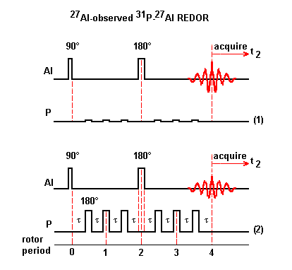
Scheme (1): Because the sample is rotating around the magic angle, the heteronuclear dipole coupling becomes time dependent and averages to zero over one rotor period. This heteronuclear dipole coupling has no effect on the ²⁷Al echo signal in a normal rotor-synchronized echo experiment.

Scheme (2): To reintroduce the effect of the heteronuclear dipole coupling, 180° pulses are applied to ³¹P nuclei which reverse the sign of the heteronuclear dipole coupling. This coupling is no longer averaged to zero over one rotor period. As a result, ²⁷Al echo signal is attenuated. 180° pulses are applied to ³¹P spins at one-half and full rotor periods after the initial 90° pulse applied to ²⁷Al spins.

As in SEDOR experiment, a normalized REDOR difference signal defined as
(ΔS)/S₀ = [signal from Scheme (1) - signal from Scheme (2)]/signal from Scheme (1),
is plotted versus the rotor periods. The interatomic distance is extracted by fitting these data with a theoretical curve.

Bertmer and Eckert proved that in the limit of short dipole evolution times where (ΔS)/S_o < 0.2 to 0.3, the REDOR curve becomes geometry-independent:
(ΔS)/S_o = (N T_r)² M₂/[I (I + 1) Pi²].

The normalized REDOR difference signal is proportional to the square of the dipole evolution time (N T_r) and the curvature depends on the van Vleck second moment M₂. The spin I is that of the non-observed (P) nuclei.

1. MS Excel 2010 macro

   The file “t1t2.dx” generated by TopSpin saves the REDOR intensities in two columns. While the first column represents an arbitrary x-scale, the measured intensities are within the second column. Remember, because of the used pulse program “redori” every odd line contains an intensity value for an REDOR spectrum (S) and every even line the corresponding intensity of the ECHO experiment (S₀).

   The following MS Excel macro calculates the values for (S₀ - S)/S₀.

   Sub redor()
   
       Dim nb_lines As Integer, half As Integer, MASrate As String
   
       nb_lines = WorksheetFunction.CountA(Columns(2))
       half = nb_lines/2
   
       MASrate = InputBox("Rotor spinning rate (Hz): ", "MASrate")
   
       For i = 1 To half
         Cells(i, 4) = (Cells(2*i, 2) - Cells(2*i - 1, 2)) / Cells(2*i, 2)
         Cells(i, 3) = (2*i) / MASrate
       Next
       
   End Sub

2. Mathematica 5 notebook 1, (ΔS)/S_o vs. N*T_r

   K. T. Mueller, Analytic solutions for the time evolution of dipolar-dephasing NMR signals, J. Magn. Reson. A 113, 81-93 (1995)

   This notebook extracts the value of the heteronuclear dipole coupling constant D from redorglycineCalphad.csv, whose left column contains the values of N*T_r, and right column those of (ΔS)/S_o.

   <<Statistics`NonlinearFit`;
   SetDirectory["C:\\Users\\pm@pascal-man.com\\Documents\\REDORglycine"];
   data = Import["redorglycineCalphad.csv."];
   data1 = Take[data, 32];
   
   sred[d_, ntr_, k_]:= 1. - BesselJ[0, Sqrt[2.] 
       d ntr]^2. + Sum[2. BesselJ[i, Sqrt[2.] d ntr]^2./(16. i^2. - 1.0), {i, 1, k}];
   
   besselfit[k_, init_] := NonlinearFit[data1,sred[d, ntr, k], ntr, {d,
   init}, AccuracyGoal -> Automatic, PrecisionGoal -> Automatic,
   ShowProgress -> True ];
   
   fit = besselfit[10, 500]
   
   tmp1 = ListPlot[data1, PlotRange -> {-0.2, 1.2}]
   
   tmp2 = Plot [fit, {ntr, 0, 0.006}, PlotRange -> {-0.2, 1.2}, Axes -> True,
       AxesOrigin -> Automatic, Axes -> Automatic]
   
   Show[tmp1, tmp2]

3. Mathematica 5 notebook 2, (ΔS)/S_o vs. N

   K. T. Mueller, Analytic solutions for the time evolution of dipolar-dephasing NMR signals, J. Magn. Reson. A 113, 81-93 (1995)

   This notebook extracts the value of D*T_r from redorglycineCalpha.csv, whose left column contains the values of N, and right column those of (ΔS)/S_o.

   <<Statistics`NonlinearFit`;
   SetDirectory["C:\\Users\\pm@pascal-man.com\\Documents\\REDORglycine"];
   data = Import["redorglycineCalpha.csv"];
   data1 = Take[data, 32];
   
   sred[n_, dtr_, k_]:= 1. - BesselJ[0, Sqrt[2.] 
       n dtr]^2. + Sum[2. BesselJ[i, Sqrt[2.] n dtr]^2./(16. i^2. - 1.0), {i, 1, k}];
   
   besselfit[k_, init_] := NonlinearFit[data1,sred[n, dtr, k], n, {dtr,
   init}, AccuracyGoal -> Automatic, PrecisionGoal -> Automatic,
   ShowProgress -> True ];
   
   fit = besselfit[10, 0.05]
   
   tmp1 = ListPlot[data1, PlotRange -> {-0.2, 1.2}]
   
   tmp2 = Plot [fit, {n, 0, 70}, PlotRange -> {-0.2, 1.2}, Axes -> True,
       AxesOrigin -> Automatic, Axes -> Automatic]
   
   Show[tmp1, tmp2]

4. Mathematica 5 notebook 3, (ΔS)/S_o (< 0.2 to 0.3) vs. N*T_r

   This notebook extracts M₂/(3π²/4) for spin I = 1/2 and (ΔS)/S_o < 0.2 to 0.3 from redorparabolD.csv, whose left column contains the values of N*T_r, and right column those of (ΔS)/S_o.

   SetDirectory["C:\\Users\\pm@pascal-man.com\\Documents"];
   data = Import["redorparabolD.csv"];
   data1 = Take[data, 4];
   
   fitresult = Fit[data1, {x^2}, x]
   
   tmp1 = ListPlot[data, PlotRange -> {-0.2, 1.2}]
   
   tmp2 = Plot [fitresult, {
       x, 0, 0.001}, PlotRange -> {-0.2, 0.4}, Axes -> True,
       AxesOrigin -> Automatic, Axes -> Automatic]
   
   Show[tmp1, tmp2]

5. Mathematica 5 notebook 4, (ΔS)/S_o (< 0.2 to 0.3) vs. N

   This notebook extracts (T_r)²M₂/(3π²/4) for spin I = 1/2 and (ΔS)/S_o < 0.2 to 0.3 from redorparabol.csv, whose left column contains the values of N, and right column those of (ΔS)/S_o.

   SetDirectory["C:\\Users\\pm@pascal-man.com\\Documents"];
   data = Import["redorparabol.csv"];
   data1 = Take[data, 4];
   
   fitresult = Fit[data1, {x^2}, x]
   
   tmp1 = ListPlot[data, PlotRange -> {-0.2, 1.2}]
   
   tmp2 = Plot [fitresult, {
       x, 0, 10}, PlotRange -> {-0.2, 0.4}, Axes -> True,
       AxesOrigin -> Automatic, Axes -> Automatic]
   
   Show[tmp1, tmp2]

6. References

   (1) Multinuclear NMR spectroscopy methods for the study of structure and dynamics in solid-state electrolytes for lithium ion batteries,
   T. Leigh Spencer Noakes,
   Advisor: Gillian R. Goward,
   (McMaster University, Canada, 2013)

   (2) Solid state NMR: AVANCE solids user manual, version 002

   (3) YouTube: Importing data into Mathematica

   (4) YouTube: Fitting data in Mathematica

   (5) YouTube: Mathematica for biologists