Rotational Echo Adiabatic Passage DOuble Resonance
Gullion proposed the REAPDOR pulse sequence to recouple the heteronuclear dipole interaction between an observed spin-1/2 and a quadrupole spin. This sequence facilitates the recoupling of quadrupole spins in Zeeman states other than ¦±1/2>.
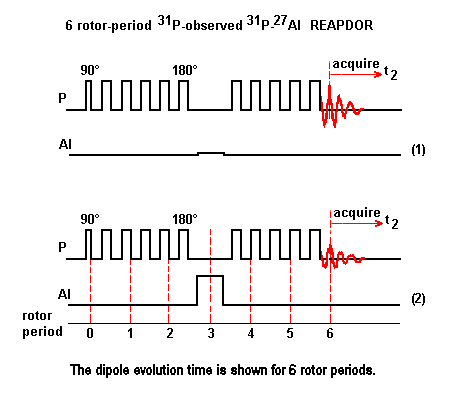
This sequence combines the REDOR approach with the adiabatic passage of TRAPDOR experiment. The dipole evolution is maintained by a REDOR train of 180° pulse applied to the observed nuclei 31P. The adiabatic passage pulse of TRAPDOR is applied to the quadrupole nuclei 27Al to less than one rotor period.
No matter the number of 180° pulses present in the dipole evolution period, there is only one adiabatic passage pulse in REAPDOR sequence.

Scheme (1): The 31P nuclei are observed with rotor-synchronized spin echo sequence consisting of multiple 180° pulses. The spacing between adjacent 180° pulse is 1/2 of the rotor period. There is no 31P pulse located at the midpoint of the dipole evolution period.
Scheme (2): The radio-frequency pulse in the 27Al channel is of duration in the order of 1/3 of the rotor period and causes a partial adiabatic population inversion, allowing the 27Al-31P dipole interaction to be recoupled and the 31P signal dephasing to be measured.
Excellent spinning speed control is necessary for REAPDOR measurement.
Usually, the REAPDOR fraction, defined by
(ΔS)/S0 = [signal from Scheme (1) - signal from
Scheme (2)]/signal from Scheme (1),
is plotted versus the dipole evolution time. The interatomic distance is
extracted by fitting these data with a theoretical curve.
The curve representing the normalized REAPDOR difference versus 27Al offset frequency allows an estimation of the quadrupole coupling constant of 27Al.
Goldbourt and coworkers demonstrated the existence of a
universal REAPDOR curve,
S1/2,5/2(nDτ) = 0.63 {1 -
exp[-(3.0 nDτ)2]} +
0.2 {1 - exp[-(0.7 nDτ)2]},
which allows estimation of distances between any observable NMR
nucleus and spin-5/2 nuclei, provided that the adiabaticity α
is greater than 0.55. With τ = 1/νR.
adiabacity parameter α = (ν1)2/νQνR
ν1 is the RF amplitude,
νR is the rotor spinning rate,
νQ = 3CQ/[2S(2S - 1)] is the quadrupole frequency,
νQ = CQ/2 for spin S = 3/2,
νQ = 3CQ/20 for S = 5/2,
νQ = CQ/14 for S = 7/2,
CQ is the quadrupole coupling constant.
Mathematica 5 notebook
This notebook extracts the value of the heteronuclear dipole coupling constant D from reapdorPAl31d.csv, whose left column contains the values of n*τ, and right column those of (ΔS)/So.
<< Statistics`NonlinearFit`;
SetDirectory["C:\\Users\\pm@pascal-man.com\\Documents"];
data = Import["reapdorPAl31d.csv"];
data1 = Take[data, 6];  (* Consider only the first six couples of values in file data *)

sred[d_, ntr_] := 0.63(1 - Exp[-(3.0 d ntr)^2]) + 0.2(1 - Exp[-(0.7d ntr)^2]);

universalfit[init_] := NonlinearFit[data1, sred[d,
      ntr], ntr, {d, init}, AccuracyGoal -> Automatic, PrecisionGoal ->
      Automatic, ShowProgress -> True]

fit = universalfit[500]

tmp1 = ListPlot[data, PlotRange -> {-0.2, 1}]

tmp2 = Plot[fit, {ntr, 0, 0.0024}, PlotRange -> {-0.2,
      1}, Axes -> True, AxesOrigin -> Automatic, Axes -> Automatic]

Show[tmp1, tmp2]
Mathematica 5 notebook
This notebook extracts the value of D*τ from reapdorPAl31.csv, whose left column contains the values of n, and right column those of (ΔS)/So.
<< Statistics`NonlinearFit`;
SetDirectory["C:\\Users\\pm@pascal-man.com\\Documents"];
data = Import["reapdorPAl31.csv"];
data1 = Take[data, 6];  (* Consider only the first six couples of values in file data *)

sred[n_, dtr_] := 0.63(1 - Exp[-(3.0 n dtr)^2]) + 0.2(1 - Exp[-(0.7n dtr)^2]);

universalfit[init_] := NonlinearFit[data1, sred[n,
      dtr], n, {dtr, init}, AccuracyGoal -> Automatic, PrecisionGoal ->
      Automatic, ShowProgress -> True]

fit = universalfit[0.05]

tmp1 = ListPlot[data, PlotRange -> {-0.2, 1}]

tmp2 = Plot[fit, {n, 0, 10}, PlotRange -> {-0.2,
      1}, Axes -> True, AxesOrigin -> Automatic, Axes -> Automatic]

Show[tmp1, tmp2]
References
YouTube: Importing data into Mathematica
YouTube: Fitting data in Mathematica
YouTube: Mathematica for biologists
(top)
