Harmonic inversion

✱ Harminv: a free program (and accompanying C library) to solve the problem of harmonic inversion: decomposing a time-series into a sum of sinusoids, including exponentially decaying sinusoids

✱ Harminv installation;
new installation procedure in cygwin-1.7 (Setup.exe version 2.738):

1 download it in your cygwin home folder
2 gzip -d harminv-1.3.1.tar.gz
3 tar -xvf harminv-1.3.1.tar
4 cd harminv-1.3.1
5 ./configure --prefix=/usr/local F77="gfortran"
6 make
7 make install

✱ Harminv manual page

✱ Harminv example

✱ sourcearchive: harminv file list

✱ Steven G. Johnson (MIT Applied Mathematics) From electrons to photons (1300 Ko MS PPT file)

✱ W. Bermel (Bruker Biospin, 2008) Fast data acquisition methods (5600 Ko PDF file)

✱ Ubuntu: harminv (1.4.1-2) [universe]

✱ CommentCaMarche: Repartitionner, installer Linux (Ubuntu 8.04), conserver Windows

✱ Avram: a virtual machine code interpreter

Harmonic inversion in Ubuntu 9.04

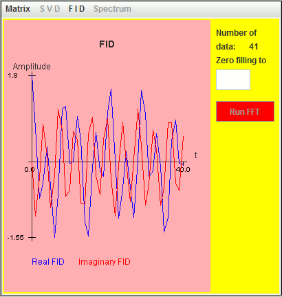
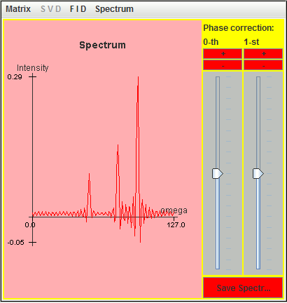
We provide OpenOffice3 spreadshead and MS Excel spreadshead which contain the real and imaginary parts of an FID associated with three Lorentzian lineshapes:

Frequency (MHz)   T2 (microsecond)   Amplitude   Phase
 0.024            4000               1           0
 0.010            3000               0.5         0
-0.010            2000               0.3         0

The FID of a Lorentzian lineshape in harminv is defined by
FID(t) = Amplitude*exp(-i*(2*π*Frequency*t - Phase))*exp(-t/T2)
FID(t) = Amplitude*exp(-i*(2*π*Frequency*t - Phase))*exp(-t*Decay)

In contrast,the FID of a Lorentzian lineshape in NMR is defined by
FID(t) = Amplitude*exp(i*(2*π*Frequency*t + Phase))*exp(-t/T2)
FID(t) = Amplitude*exp(i*(2*π*Frequency*t + Phase))*exp(-t*Decay)

Decay (= 1/T2) and Frequency define the quality factor Q:
Q = π*|Frequency|/Decay = π*|Frequency|*T2
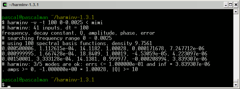
10 is the value by default of Q.

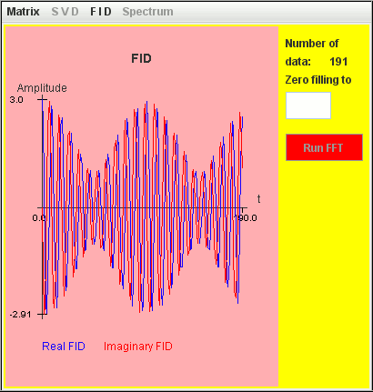
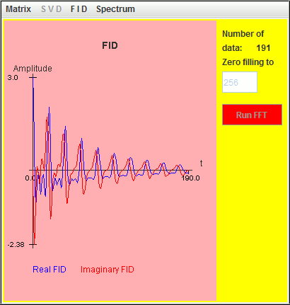
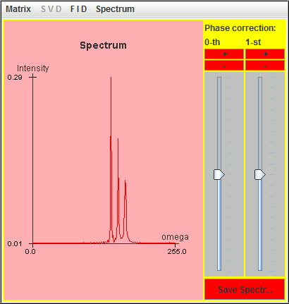
This FID and the corresponding spectrum are represented in the following two figures:

We select the spreadsheet cells containing the real and imaginary parts of this FID, and then paste the data into a text file saved as mimi. In this file, the character i is appended to the imaginary part; the real and imaginary parts of an amplitude are joined.

Within a spectral width SW (= 1/DW) ranging from -SW/2 to SW/2, only spectrum lines located inside ]-SW/4, SW/4[ are identified by harminv, including folded spectrum lines.

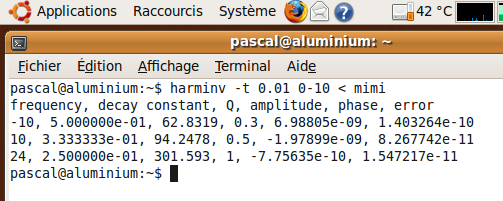
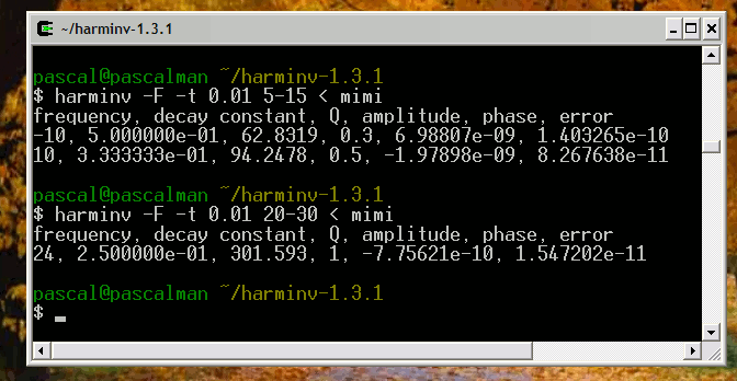
In Ubuntu operating system, the results provided by harminv are:

Harmonic inversion in Cygwin 1.5

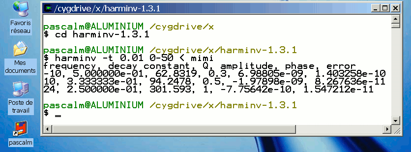
In MS Windows, use Bloc-notes or WordPad for saving the text file mimi.

For the other data, see Harmonic inversion in Ubuntu

Effect of spin-spin relaxation time T2 in harminv

Example 1

Consider another simulation with two Lorentzian lineshapes where both T2 = 400 seconds:

Frequency (Hz)    T2 (second)   Amplitude
 1                400               1
 1.1              400               2

The signal FID is generated with a step t = 0.1 second.

The two signals are detected by harminv.

Example 2

Consider the same simulation but both T2 = 4 seconds:

Frequency (Hz)    T2 (second)   Amplitude
 1                4                 1
 1.1              4                 2

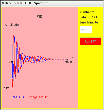
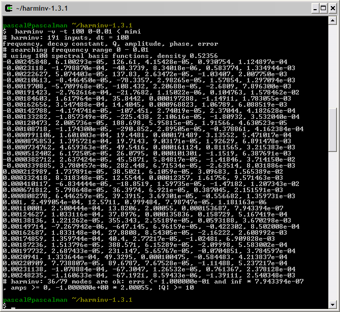
This figure shows that within a spectral width SW = 10 Hz ranging from -5 Hz to +5 Hz, only spectrum lines located inside ]-2.5 Hz, 2.5 Hz[ are identified by harminv.

The two signals are detected by harminv.

Example 3

Consider the same simulation but T2 = 4 seconds for the low frequency Lorentzian lineshape and T2 = 2 seconds for the high frequency Lorentzian lineshape :

Frequency (Hz)    T2 (second)   Amplitude
 1                4                 1
 1.1              2                 2

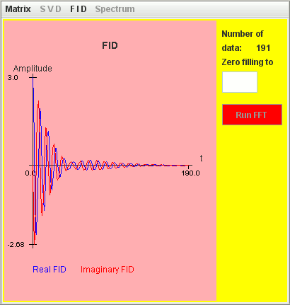
Only the signal with T2 = 4 seconds is detected by harminv.

Example 4

Consider the same simulation but T2 = 2 seconds for the low frequency Lorentzian lineshape and T2 = 4 seconds for the high frequency Lorentzian lineshape :

Frequency (Hz)    T2 (second)   Amplitude
 1                2                 1
 1.1              4                 2

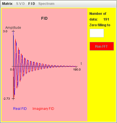
Only the signal with T2 = 4 seconds is detected by harminv.

Example 5

Consider the same simulation but both T2 = 2 seconds:

Frequency (Hz)    T2 (second)   Amplitude
 1                2                 1
 1.1              2                 2

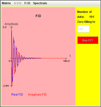
The two signals are not detected by harminv.

Since the quality factor Q of a signal is proportional to T2, it decreases with T2. When Q is lower than its default value (= 10), this signal is not detected by harminv. Fortunately, we can decrease the default value of Q.

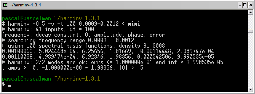
Once we define the default value of Q to 5, the two signals are detected by harminv.

Effect of frequency offset in harminv

Example 1

Consider another simulation with three Lorentzian lineshapes where T2 = 8 seconds:

    Frequency (Hz)    T2 (second)   Amplitude
 0.5              8               1
 1.0              8               1
 1.5              8               1

The signal FID is generated with a step t = 0.1 second.
The frequency axis in harminv increases from left to right 
direction.

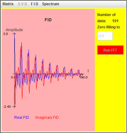
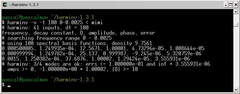
The three signals located at 0.5 Hz, 1 Hz, and 1.5 Hz are detected by harminv. The Q value (= 12.5671) of the 0.5-Hz signal is close to the default value (= 10 ).

Example 2

Consider the same simulation with three Lorentzian lineshapes where T2 = 6 seconds:

Frequency (Hz)    T2 (second)   Amplitude
 0.5              6               1
 1.0              6               1
 1.5              6               1

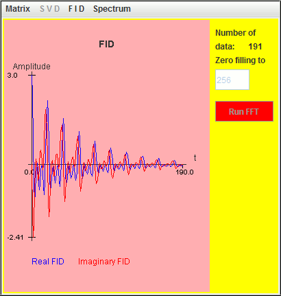
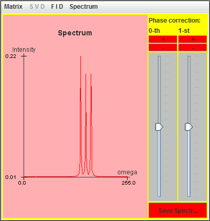
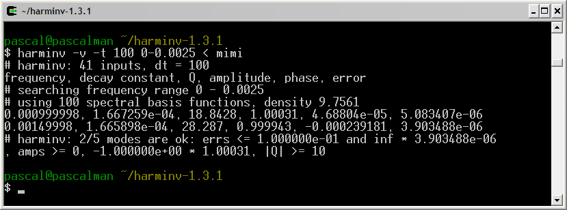
Only two signals (1 Hz and 1.5 Hz) are detected by harminv. That located at the lowest frequency (0.5 Hz) is missing due to T2 value. Its Q value is less than 10.

Example 3

Consider the same simulation with three Lorentzian lineshapes where T2 = 3 seconds:

Frequency (Hz)    T2 (second)   Amplitude
 0.5              3               1
 1.0              3               1
 1.5              3               1

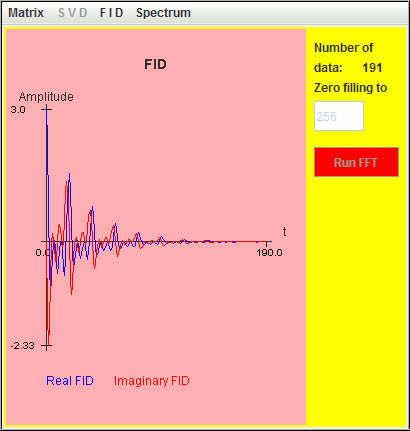
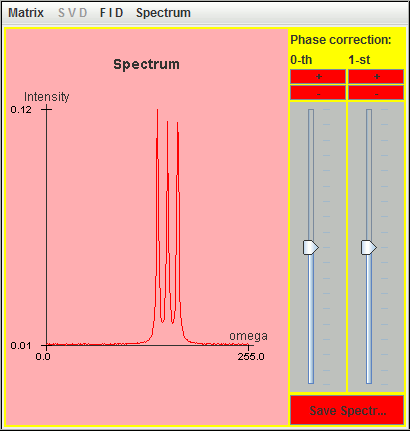
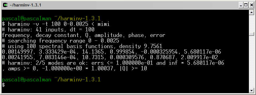
Only the signal located at the highest frequency (1.5 Hz) is detected by harminv. The other two located at lower frequencies (0.5 Hz and 1 Hz) are missing due to T2 value.

Example 4

Consider the same simulation with three Lorentzian lineshapes of different T2:

Frequency (Hz)    T2 (second)   Amplitude
 0.5              9               1
 1.0              6               1
 1.5              3               1

Since the value of T2 increases when the frequency offset decreases, the Q values of the three signals remain larger than the default value (= 10). As a result, the three signals are detected by harminv.

Dead time correction in harminv

FID simulation with SIMPSON

We provide OpenOffice3 spreadshead and MS Excel spreadshead which contain the real and imaginary parts of an FID simulated with SIMPSON. This FID is generated with a step t = 0.1 millisecond. The following figure is the absorption spectrum.

This FID is analyzed with harminv:

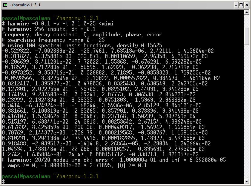
Among these results, we choose the nine most significant lineshapes:

pascal@pascalman ~/harminv-1.3.1
$ harminv -Q 0.1 -t 0.1 0-25 < mimi

frequency,  decay constant, Q,        amplitude,  phase,      error
-0.206699,  8.411231e-02,   7.72022,  1.55368,    -0.676291,  6.592080e-05
-0.18529,   3.717283e-01,   1.56595,  1.62323,    -0.362238,  2.716799e-03
-0.0973252, 9.353716e-01,   0.326882, 2.71895,    -0.0858323, 1.759053e-02
0.0212417,  1.395977e-01,   0.478036, 0.0325433,   0.630549,  2.242755e-02
0.127801,   2.072755e-01,   1.93703,  0.0895102,   2.44031,   3.941283e-03
0.174193,   9.237603e-01,   0.59241,  2.07773,     0.306538,  2.054223e-02
0.23999,    2.132489e-01,   3.53555,  0.0751803,  -1.5363,    2.368882e-03
0.381661,   5.100819e-01,   2.35065,  0.857901,    0.878896,  3.941438e-03
0.416107,   1.574062e-01,   8.30487,  0.237168,    1.50239,   5.907249e-04

The following figure is the corresponding spectrum simulated with these nine most significant lineshapes.

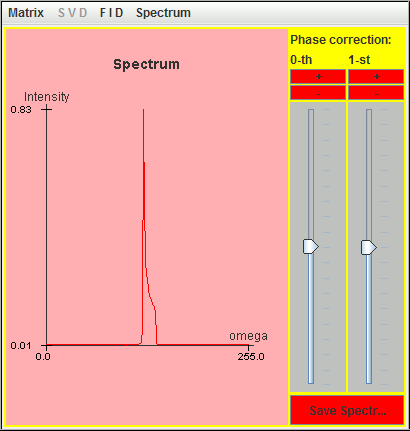
Dead time of an FID simulated with SIMPSON

We delete the first ten complex points of the previous FID simulated with SIMPSON. The following figure is the corresponding spectrum.

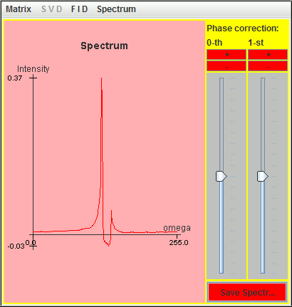
This truncated FID is analyzed with harminv:

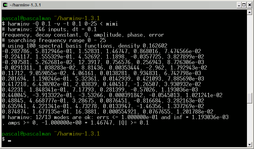
Among these results, we choose the nine most significant lineshapes:

pascal@pascalman ~/harminv-1.3.1
$ harminv -Q 0.1 -t 0.1 0-25 < mimi

frequency,  decay constant, Q,        amplitude,  phase,     error
-0.282786,  5.812946e-01,   1.52831,  1.46747,    0.868016,  7.474566e-02
-0.224117,  1.555329e-01,   4.52692,  1.1898,    -0.0357725, 3.827899e-02
-0.207581,  5.262681e-02,   12.3917,  0.756576,   0.256943,  8.726306e-03
0.11712,    9.059055e-02,   4.06161,  0.0138281,  0.934831,  6.742798e-03
0.201694,   1.190246e-01,   5.32361,  0.0142939,  0.421093,  7.885690e-03
0.417218,   6.430202e-01,   2.03839,  0.404517,  -1.26507,   3.930932e-02
0.42231,    1.848341e-01,   7.17793,  0.281399,  -0.57026,   1.193036e-03
0.48845,    4.668777e-01,   3.28675,  0.0876451, -0.816684,  3.282163e-02
0.635941,   4.221341e-01,   4.73278,  0.0133947, -1.46356,   1.337269e-02

The following figure is the corresponding spectrum simulated with these nine most significant lineshapes.

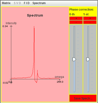
Correction of dead time of an FID simulated with SIMPSON

Thanks to these nine lineshapes, we simply simulate the ten missing complex points of the previous truncated FID simulated with SIMPSON. The following figure is the corresponding spectrum.

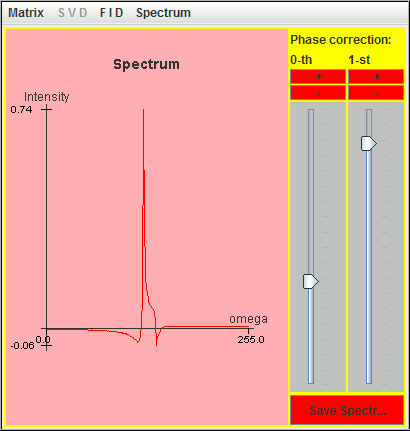
The recovered lineshape is not perfect but the effect of dead time has been attenuated.

Harmonic inversion - reference

✱ Indranil Ghosh, Subhayan Chakraborty, Shalini Pandey, and Arindam Ghosh
Diagonal free processing of conventional phase sensitive COSY using Filter Diagonalization Method,
ChemRxiv (2022).
Open access

✱ Claudio José Magon, José Fernando Lima, Ronny Rocha Ribeiro, and Mateus José Martins
The harmonic inversion of the field-swept fixed-frequency resonance spectrum,
J. Magn. Reson. 184, 176-183 (2007).
Abstract

✱ Elizabeth A. O'Sullivan and Colin F. N. Cowan
Harmonic inversion of room impulse response signals,
The Institute of Mathematics and its Applications (2006).

✱ Sharif D. Kunikeev, Erdinç Atilgan, Howard S. Taylor, Alexey L. Kaledin, and Jörg Main
An application of error reduction and harmonic inversion schemes to the semiclassical calculation of molecular vibrational energy levels,
J. Chem. Phys. 120, 6478 (2004).
Abstract

✱ Vladimir A. Mandelshtam
On harmonic inversion of cross-correlation functions by the filter diagonalization method,
J. Theor. Comput. Chem. 2, 1-9 (2003).
PDF

✱ V. A. Mandelshtam
FDM: the filter diagonalization method for data processing in NMR experiments,
Prog. Nucl. Magn. Reson. Spectrosc. 38, 159-196 (2001).
Abstract

✱ Thomas Bartsch, Jörg Main, and Günter Wunner
Semiclassical quantization by harmonic inversion: Comparison of algorithms,
Phys. Rev. E 64, 056705/1-056705/5 (2001).

✱ J. Main, P. A. Dando, Dz Belkic, and H. S. Taylor
Decimation and harmonic inversion of periodic orbit signals,
J. Phys. A: Math. Gen. 33, 1247-1263 (2000).
Abstract

✱ J. Main
Use of harmonic inversion techniques in semiclassical quantization and analysis of quantum spectra,
Phys. Rep. 316, 233-338 (1999).
Abstract (Abstract)

✱ Gunnar Jeschke, Vladimir A. Mandelshtam, and A. J. Shaka
Pure absorption electron spin echo envelope modulation spectra by using the filter-diagonalization method for harmonic inversion,
J. Magn. Reson. 137, 221-230 (1999).

✱ Rongqing Chen and Hua Guo
Efficient calculation of matrix elements in low storage filter diagonalization,
J. Chem. Phys. 111, 464-471 (1999).
Abstract

✱ P. A. Houle, N.-G. Zhang, and C. L. Henley
Semiclassical mechanics of a nonintegrable spin cluster,
Phys. Rev. B 60, 15179-15186 (1999).
Abstract

✱ Haitao Hu, Que N. Van, Vladimir A. Mandelshtam, and A. J. Shaka
Reference deconvolution, phase correction, and line listing of NMR spectra by the 1D Filter Diagonalization Method,
J. Magn. Reson. 134, 76-87 (1998).
Abstract

✱ John W. Pang, Thorsten Dieckmann, Juli Feigon, and Daniel Neuhauser
Extraction of spectral information from a short-time signal using filter-diagonalization: Recent developments and applications to semiclassical reaction dynamics and nuclear magnetic resonance signals,
J. Chem. Phys. 108, 8360-8368 (1998).
Abstract

✱ Vladimir A. Mandelshtam and Howard S. Taylor
Multidimensional harmonic inversion by filter-diagonalization,
J. Chem. Phys. 108, 9970-9977 (1998).
Abstract

✱ Frank Grossmann, Vladimir A. Mandelshtam, Howard S. Taylor, and John S. Briggs
Harmonic inversion of semiclassical short time signals,
Chem. Phys. Lett. 279, 355-360 (1997).
Abstract

✱ V. A. Mandelshtam and H. S. Taylor
Harmonic inversion of time signals and its applications,
J. Chem. Phys. 107, 6756-6769 (1997).
Abstract
Erratum, ibid. 109, 4128 (1998).
Abstract

✱ Jörg Main, Vladimir A. Mandelshtam, and Howard S. Taylor
Periodic orbit quantization by harmonic inversion of Gutzwiller's recurrence function,
Phys. Rev. Lett. 74, 825-828 (1997).

✱ John W. Pang and Daniel Neuhauser
Application of generalized filter-diagonalization to extract instantaneous normal modes,
Chem. Phys. Lett. 252, 173-180 (1996).
Abstract

✱ Michael R. Wall and Daniel Neuhauser
Extraction, through filter-diagonalization, of general quantum eigenvalues or classical normal mode frequencies from a small number of residues or a short-time segment of a signal. I. Theory and application to a quantum-dynamics model,
J. Chem. Phys. 102, 8011-8022 (1995).
Abstract

✱ Dževad Belkić: Quantum-Mechanical Signal Processing and Spectral Analysis, Institute of Physics Publishing, 2004; ISBN: 9780750310192

✱ John R. Sabin (Series Editor), Erkki J. Brandas (Series Editor): Advances in Quantum Chemistry, Volume 56, Academic Press, 2009; ISBN-10: 0123747805; ISBN-13: 978-0123747808

Harmonic inversion - author

✱ Howard S. Taylor, University of Southern California

✱ Vladimir A. Mandelshtam, University of California, Irvine

Generalized eigenvalue problem

✱ GNU Scientific Library: Reference manual

✱ Mike Brookes: The matrix reference manual

✱ Wikipedia: Eigendecomposition of a matrix

✱ Wikipedia: Matrix decomposition

✱ Wikipedia: Schur decomposition

✱ LAPACK users' guide, Third edition: Eigenvalues, eigenvectors and generalized Schur decomposition

✱ LAPACK users' guide, Third edition: Generalized Nonsymmetric Eigenproblems (GNEP)

✱ Templates for the Solution of Algebraic Eigenvalue Problems: QZ algorithm

✱ Jack Dongarra: CRC-LAPACK-2005

Generalized eigenvalue problem - reference

✱ David S. Watkins: Performance of the QZ algorithm in the presence of infinite eigenvalues,
SIAM J. Matrix Anal. Appl 22, 364-375 (2000).
Abstract

✱ Krister Dackland and Bo KÃ¥gström: Reduction of a regular matrix pair (A, B) to block Hessenberg-triangular form,
Book Series: Lecture Notes in Computer Science, 1041, 125-133 (1996).
Book: Applied Parallel Computing Computations in Physics, Chemistry and Engineering Science,
Abstract, Abstract

✱ J. H. Wilkinson: Kronecker's canonical form and the QZ algorithm,
Linear Algebra Appl. 28, 285-303 (1979).
Abstract

✱ Burton S. Garbow: ALGORITHM 535 The QZ algorithm to solve the generalized eigenvalue problem for complex matrices [F2],
ACM Trans. Math. Software (TOMS) 4, 404-410 (1978).
Abstract

✱ B. S. Garbow, J. J. Dongarra, J. M. Boyle , and C. B. Moler: Matrix Eigensystem Routines — EISPACK Guide Extension,
Book Series: Lecture Notes in Computer Science, 51 (1977).
Abstract

✱ Robert C. Ward: The combination shift QZ algorithm,
SIAM J. Numer. Anal. 12, 835-853 (1975).
Abstract

✱ Linda Kaufman: ALGORITHM 496 The LZ algorithm to solve the generalized eigenvalue problem for complex matrices [F2],
ACM Trans. Math. Software (TOMS) 1, 271-281 (1975).
Abstract

✱ Linda Kaufman: The LZ-algorithm to solve the generalized eigenvalue problem,
SIAM J. Numer. Anal. 11, 997-1024 (1974).
Abstract

✱ C. B. Moler and G. W. Stewart: An algorithm for generalized matrix eigenvalue problems,
SIAM J. Numer. Anal. 10, 241-256 (1973).
Abstract

Generalized eigenvalue problem - book

✱ Gilbert. W. Stewart: Matrix Algorithms, Volume II: Eigensystems
SIAM (2001).
Abstract

✱ Vasile Sima: Algorithms for Linear-Quadratic Optimization,
Series: Pure and Applied Mathematics
Marcel Dekker (2001).
Abstract

✱ Gene Howard Golub, Charles F. Van Loan: Matrix Computations, third edition
The Johns Hopkins University Press (1996).
Abstract

✱ James Hardy Wilkinson: The Algebraic Eigenvalue Problem,
Oxford University Press (1988).
Abstract

✱ Y. Saad: Numerical Methods for Large Eigenvalue Problems,
Manchester University Press Series in Algorithms and Architectures for Advanced Scientific Computing
Pages 1-99, 100-199, 200-299, and 300-347

✱ Hang T. Lau: A Numerical Library in Java for Scientists and Engineers, CRC Press, 2003; ISBN: 1584884304

Linux OS

✱ Système d'exploitation basé sur Linux : Fedora

✱ Mauriat Miranda: Download Fedora Linux

✱ Softpedia: Installing Fedora 8 Werewolf

✱ InformIT: Installing Fedora

✱ UNIX tutorial for beginners

✱ PCWDLD: Linux commands cheat sheet as quick reference for both experienced and basic users.

✱ GNU Operating System

✱ GCC: the GNU Compiler Collection

✱ David Henry: Une introduction à  GCC et MinGW

✱ ubuntu-fr.org: Comment utiliser MingW32 pour faire des exécutables Windows ?

✱ GNU C library

Cygwin

✱ Wikipedia: Cygwin is free software that provides a Unix-like environment and command-line interface for Microsoft Windows

✱ George B. Moodya: An introduction to Cygwin
Cygwin consists of a Unix system call emulation library, cygwin1.dll, together with a vast set of GNU and other free software applications organized into a large number of optional packages

✱ Cygwin information and installation

✱ Cygwin installation on Windows XP

✱ InOnIt: Cygwin and Java

✱ Cygwin: Programmation

✱ Jacques Grelet: Cygwin

LPSVD

✱ BRUKER BIOSPIN Newsletter (PDF): NMR processing technique “Linear Prediction”

✱ Miroslav ŠTĚPÁN: LPSVD algorithm for parameter estimation of damped sinusoids, (PDF)

✱ CaltechBOOK: The theory of linear prediction
Vaidyanathan, P. P. (2008) The theory of linear prediction. Synthesis Lectures on Signal Processing (3). Morgan & Claypool. ISBN 9781598295764

✱ Jeffrey C. Hoch, Mark W. Maciejewski, and Michael R. Gryk
Comment on "Magnetic resonance spectroscopy identifies neural progenitor Cells in the live human brain",
Science 321, 640 (2008).
Abstract

✱ Louis N. Manganas, Xueying Zhang, Yao Li, Raphael D. Hazel, S. David Smith, Mark E. Wagshul, Fritz Henn, Helene Benveniste, Petar M. Djuric, Grigori Enikolopov, and Mirjana Maletic-Savatic
Magnetic resonance spectroscopy identifies neural progenitor cells in the live human brain,
Science 318, 980-985 (2007).
Abstract

✱ Yun-Wei Chiang, Antonio Costa-Filho, and Jack H. Freed
2D-ELDOR using full S_c- fitting and absorption lineshapes,
J. Magn. Reson. 188, 231-245 (2007).

✱ Y. K. Lee, R. L. Vold, G. L. Hoatson, Y.-Y. Lin, and A. Pines
Linear prediction with singular-value decomposition for removing phase artifacts in 2D VACSY spectra,
J. Magn. Reson. A 112, 112-117 (1995).

✱ A. Diop, A. Briguet, and D. Graveron-Demilly
Automatic in vivo NMR data processing based on an enhancement procedure and linear prediction method,
Magn. Reson. Med. 27, 318-328 (1992).

✱ David S. Stephenson
Linear prediction and maximum entropy methods in NMR spectroscopy,
Prog. Nucl. Magn. Reson. Spectrosc. 20, 515-626 (1988).
Abstract

✱ H. Barmuijsen, R. de Beer, W. M. M. J. Bovee, J. H. N. Creyghton, and D. van Ormondt
Application of linear prediction and singular value decomposition (LPSVD) to determine NMR frequencies and intensities from the FID,
Magn. Reson. Med. 2, 86-89 (1985).
Abstract

✱ Ramdas Kumaresan and Donald. W. Tufts
Estimating the parameters of exponentially damped sinusoids and pole-zero modeling in noise,
IEEE Trans. Acoust. Speech Signal Process. ASSP 30, 833-840 (1982).